binfalse
Stupid handycrafts
April 12th, 2011Today I had to install a new server for some biologists, they want to do some NGS. It took a whole day and all in all we’ll send it back…
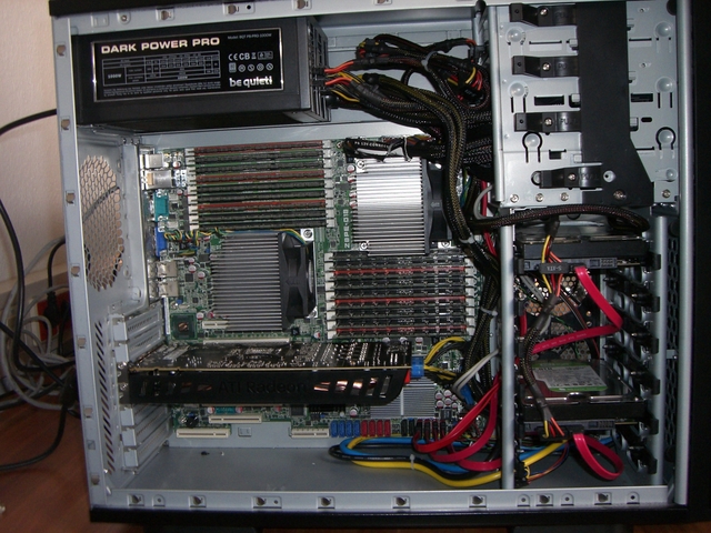
These biologists ordered the server without asking us, I think the salesmen noticed that they don’t have expertise. The money is provided by the university, so no need to design for efficiency. And that is how it came that they send the hardware (2 Xeon-DP 5500, 72 GB mem) in a desktop case with a Blu-ray writer, a DVD-writer, a GPU with 2.72 TeraFLOPS (afaik they don’t want to OpenCL) and: NO CHASSIS FANS!! Ouch..
It’s as clear as daylight that this cannot work. Did they thought the hot air around the mem (18 slots, each 4GB) leaves the chassis by diffusion?? The processor cooling construction for my Athlon X2 is twice as big as all their fans together…
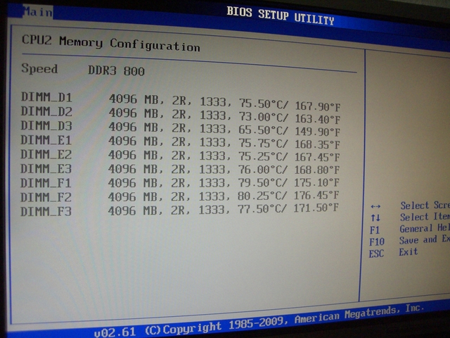
After setting up a Linux and installing lm-sensors the CPU’s are running at >75°C, fighting for air. Of course we immediately turned off the hardware! After half an hour we were able to start it again and took a look at the BIOS sensors for the memory. No time to get bored while the temperatures raised up to 80°C and more in less than 5 min, see figure 2… Of course time to turn it off again! Don’t want to hazard a nuclear meltdown..
They also enclosed a raid controller. I’ve googled that. Less than 100$.. wtf… The controller came with a CD to create a driver disk. But when you boot into the small Linux on the CD it hangs with the message “Searching for CD…”. And there is no driver for us, you are only able to use this controller when you are running Win 2003/XP/Vista or a RHEL or a Suse Enterprise. Other systems are not supported.. Proprietary crap..
What should I say, I’m pissed off. A whole business day is gone for nothing… Just because of some less-than-commodity handycrafts… I strongly recommend to ask Micha before plugging such bullshit!
Closer look to Triwave and MSE
April 9th, 2011After getting started to work with the new Synapt G2 HDMS from Waters a few questions about the working principle of this machine came up. Here I’ll try to explain where the drift time detector is located and how the software can distinguish between fragments produced in the trap and transfer cell, respectively.
As far as I know Waters is the first manufacturer who joined the IMS- and QTOF-technologies to combine all well known benefits from the QTOF instruments plus the advantages of separating ions by their shape and size.
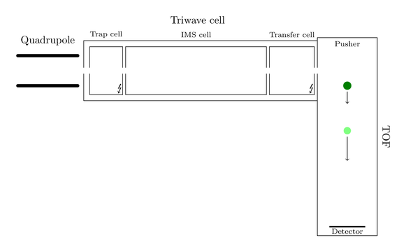
But lets start at the beginning. As any other MS instrument the Synapt carries an ion source. Here are also some attractive innovations located, but nothing remarkable for now, so I won’t explain anything of it. The interesting magic part starts when the ions pass the quadrupole. To give you a visual feedback of my explanations I created an image of the hierarchical ion path:

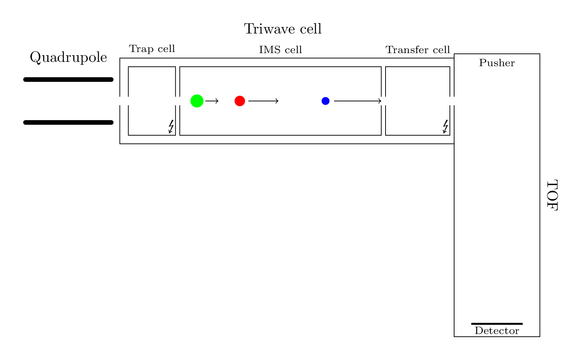
Assume only one big black ion has entered the machine and found its way to the quadrupole. This ion will now follow the ion path and arrive at the Triwave cell, consisting of a trap cell, the new IMS cell and a transfer cell. Trap and transfer cell are able to fragment the ions, so you can produce fragments before and/or after separation by ion mobility. Producing fragments is nothing new, most of the MS instruments out there are able to do so.
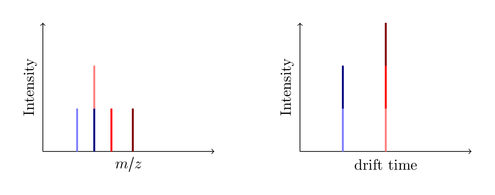
So consider this big black ion is decayed in the trap cell into three smaller ions, a blue, a red and a green one:
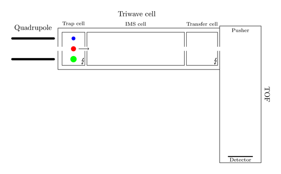
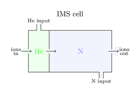
As the figure indicates all fragments have different shape sizes and actually share the same velocity. They now enter the magic IMS cell and an IMS cycle starts. This cell is a combination of two chambers. One small chamber at the front of this cell is flooded with helium and operates as a gate. During an IMS cycle it is impossible that further ions can pass this gate. The main chamber of the IMS cell is filled with nitrogen. The pressures of helium and nitrogen are sensible tuned, such that nitrogen doesn’t form an counterflow for incoming ions. Here is a smart graphic of both chambers:
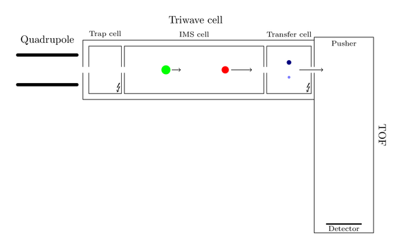
These nitrogen molecules represent a barrier, so the passing ions are slowed done while they have to find their way through this chamber. Here is the awesome trick located! The bigger the ion shape the bigger the braking force and the slower the ion. A heavy but compact ion might be faster than a lightweight but space consuming ion. So the drift time through the IMS cell is independent of m/z values, it separates the ions by their shape size. Back to the example the blue ion is much smaller so it is much faster, in contrast the fat green ion is inhibited a lot by this nitrogen gas:
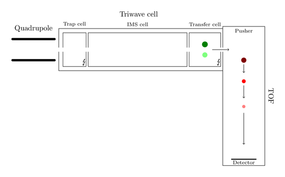
Thence the blue fragment arrives first at the transfer cell. Here it is again fragmented in smaller components:
Each of the smaller blue ions then reaches the TOF analyzer. Here they have to fly a specific way, the required time is tracked at the TOF-detector. Heavier ions are slower, so the resulting m/z values are measured here:

The first acquired spectrum is recorded. All blue ions have the same drift time (they were all present when the pusher pushed), but are distinguished by their mass:
At the same time the red ion was able to reach the transfer cell and got also decayed again. Passing the transfer cell they reach the pusher and the next push will make them fly through the flight tube:
All red fragments also have the same drift time, but this time differs from the drift time of the blue ions. Nothing was said about their mass, the m/z isn’t determined before their flight through the TOF analyzer! So it might (and will) happen, that they are lighter than the blue ions. At this point the spectrum will look like this:
The same will happen with the green ions. Entering transfer cell, getting decayed, flying with the next push:
At the end the spectrum produced by the big black ion might look like this:
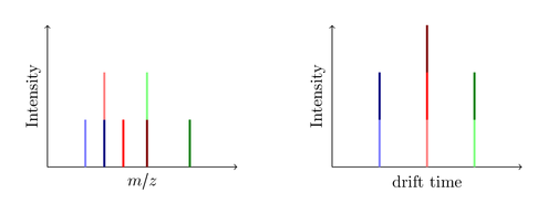
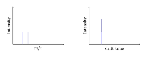
You see, the drift time is measured without any additional IMS detector! A common MS instrument is just able to record the left m/z spectrum, so if it produces the same seven fragments you are only able to identify five peaks. Since the dark blue and the light red ions have the same mass (they are called isobars) the produced peak is a merge of both ions. Same issue with the dark red and the light green ion. The new IMS technology now enables you to split this peak by the required drift time. Nice, isn’t it?
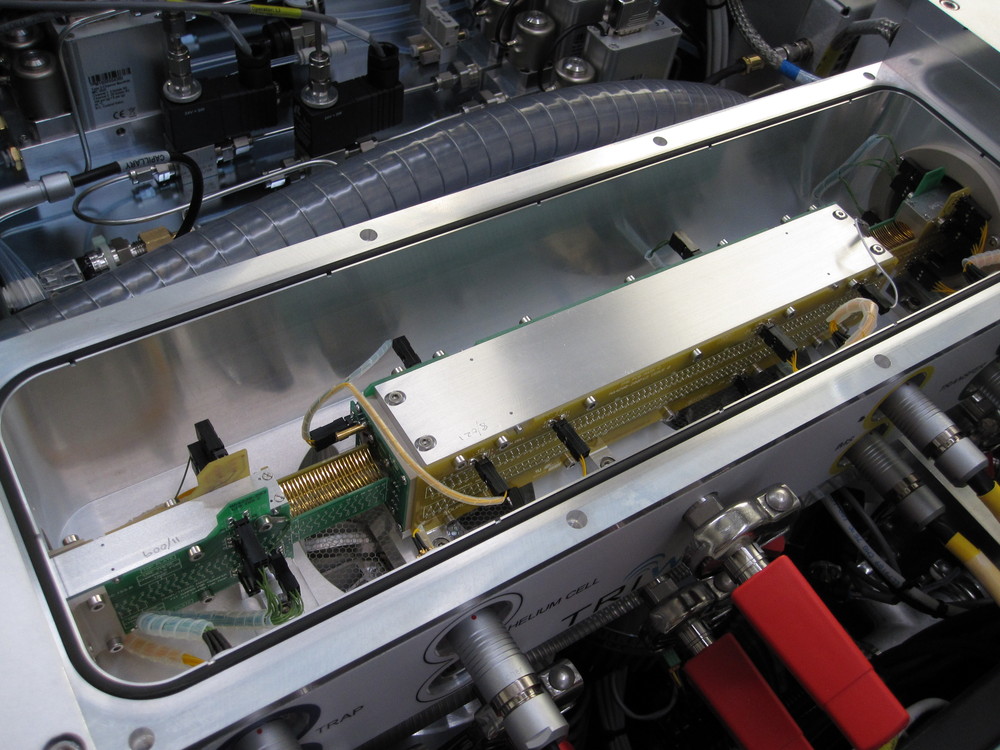
Ok, so far, back to reality! First of all I have to say the images are not true to scale, I’ve warped the elements for a better representation. The size of the IMS cell is not comparable with the size of the TOF! Fortunately the IMS cell was broken so I was able to look into the machine (figure 1). While the TOF is about 1m the IMS cell is a bit longer than half of a keyboard length, see figure 2. By the way the ions don’t fly a linear way through the TOF analyzer. The Synapt operates with reflectrons and knows two modes: V-TOF (ions are reflected once) and W-TOF (ions are reflected three times).
The energy beam transporting the ions through the IMS cell can be understood as a wave. You can define the wave height and the velocity to effectively separate your present ions. Don’t ask me why the call it height and velocity, and not amplitude and frequency, but what ever ;-) These two parameter are nevertheless very sensitive. So if they are not chosen very well, an ion might need longer then one IMS cycle to pass the cell, so it enters the transfer cell when the next cycle is still started. I don’t have any empirical knowledge yet, but it seems to be hard to find a well setting.
The complexity of this system of curse increases crucial if there isn’t only one big black ion in your machine! So analyzing is not that trivial as my images might induce. You are also able to separately enable or disable fragmentation in trap and transfer cell. So your awareness of this process is essential to understand the resulting data.
In reality one IMS cycle takes the time of 200 pushes, but the pusher isn’t synchronized with the IMS gate. What did he say? Time to get confused! If an IMS cycle takes exactly the time of 200 pushes, ions that arrive between two pushes (one push of course takes some time) should be lost every time, because they should arrive with the next IMS cycle, exactly +200 pushes, again between two pushes. This scenario would mean your sensitivity is crap. Theoretically correct, but fortunately we can’t count on our hardware. Even if you tell the pusher to push every 44 μs, the consumed time will fluctuate in the real world. So he’ll need 45 μs for one push and 43.4 μs for the following. Instead an IMS cycle will always take 44*200=8800 μs, independent of the real time the pusher needs for 200 pushes. So if an IMS cycle starts exactly with a push the next cycle will probably start within two pushes and ions that weren’t able to catch a push last time might now get pushed.
All in all you have to agree that this is an absolutely great invention. If you are interested in further information Waters provides some videos to visualize the IMS technology, and here you can find some smart pictures of the Triwave system in a Synapt.
Comparison of compression
April 4th, 2011I recently wrote an email with an attached LZMA archive. It was immediately answered with something like:
What are you doing? I had to boot linux to open the file!
First of all I don’t care whether user of proprietary systems are able to read open formats, but this answer made me curious to know about the differences between some compression mechanisms regarding compression ratio and time. So I had to test it!
This is nothing scientific! I just took standard parameters, you might optimize each method on its own to save more space or time. Just have a look at the parameter -1..-9 of zip. But all in all this might give you a feeling for the methods.
Candidates
I’ve chosen some usual compression methods, here is a short digest (more or less copy&paste from the man pages):
- gzip: uses Lempel-Ziv coding (LZ77), cmd:
tar czf $1.pack.tar.gz $1 - bzip2: uses the Burrows-Wheeler block sorting text compression algorithm and Huffman coding, cmd:
tar cjf $1.pack.tar.bz2 $1 - zip: analogous to a combination of the Unix commands tar(1) and compress(1) and is compatible with PKZIP (Phil Katz’s ZIP for MSDOS systems), cmd:
zip -r $1.pack.zip $1 - rar: proprietary archive file format, cmd:
rar a $1.pack.rar $1 - lha: based on Lempel-Ziv-Storer-Szymanski-Algorithm (LZSS) and Huffman coding, cmd:
lha a $1.pack.lha $1 - lzma: Lempel-Ziv-Markov chain algorithm, cmd:
tar --lzma -cf $1.pack.tar.lzma $1 - lzop: imilar to gzip but favors speed over compression ratio, cmd:
tar --lzop -cf $1.pack.tar.lzop $1
All times are user times, measured by the unix time command. To visualize the results I plotted them using R, compression efficiency at X vs. time at Y. The best results are of course located near to the origin.
Data
To test the different algorithms I collected different types of data, so one might choose a method depending on the file types.
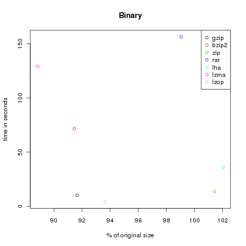
Binaries
The first category is called binaries. A collection of files in human-not-readable format. I copied all files from /bin and /usr/bin , created a gpg encrypted file of a big document and added a copy of grml64-small_2010.12.iso. All in all 176.753.125 Bytes.
| Method | Compressed Size | % of original | Time in s |
|---|---|---|---|
| gzip | 161.999.804 | 91.65 | 10.18 |
| bzip2 | 161.634.685 | 91.45 | 71.76 |
| zip | 179.273.428 | 101.43 | 13.51 |
| rar | 175.085.411 | 99.06 | 156.46 |
| lha | 180.357.628 | 102.04 | 35.82 |
| lzma | 157.031.052 | 88.84 | 129.22 |
| lzop | 165.533.609 | 93.65 | 4.16 |
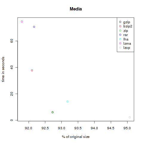
Media
This is a bunch of media files. Some audio data like the I have a dream-speech of Martin-Luther King and some music. Also video files like the The Free Software Song and Clinton’s I did not have sexual relations with that woman are integrated. I attached importance to different formats, so here are audio files of the type ogg, mp3 mid, ram, smil and wav, and video files like avi, ogv and mp4. Altogether 95.393.277 Bytes.
| Method | Compressed Size | % of original | Time in s |
|---|---|---|---|
| gzip | 88.454.002 | 92.73 | 6.04 |
| bzip2 | 87.855.906 | 92.10 | 37.82 |
| zip | 88.453.926 | 92.73 | 6.17 |
| rar | 87.917.406 | 92.16 | 70.69 |
| lha | 88.885.325 | 93.18 | 14.22 |
| lzma | 87.564.032 | 91.79 | 74.76 |
| lzop | 90.691.764 | 95.07 | 2.28 |
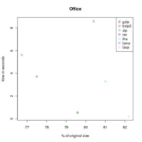
Office
The next category is office. Here are some PDF from different journals and office files from LibreOffice and Microsoft’s Office (special thanks to @chschmelzer for providing MS files). The complete size of these files is 10.168.755 Bytes.
| Method | Compressed Size | % of original | Time in s |
|---|---|---|---|
| gzip | 8.091.876 | 79.58 | 0.55 |
| bzip2 | 8.175.629 | 80.40 | 8.58 |
| zip | 8.092.682 | 79.58 | 0.54 |
| rar | 7.880.715 | 77.50 | 3.72 |
| lha | 8.236.422 | 81.00 | 3.29 |
| lzma | 7.802.416 | 76.73 | 5.62 |
| lzop | 8.358.343 | 82.20 | 0.21 |
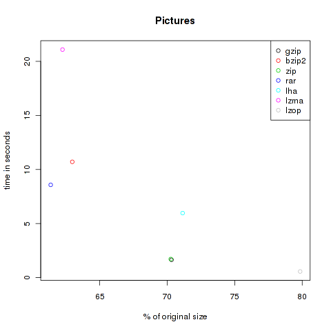
Pictures
To test the compression of pictures I downloaded 10 files of each format bmp, eps, gif, jpg, png, svg and tif. That are the first ones I found with google’s image search engine. In total 29’417’414 Bytes.
| Method | Compressed Size | % of original | Time in s |
|---|---|---|---|
| gzip | 20.685.809 | 70.32 | 1.65 |
| bzip2 | 18.523.091 | 62.97 | 10.71 |
| zip | 20.668.602 | 70.26 | 1.72 |
| rar | 18.052.688 | 61.37 | 8.58 |
| lha | 20.927.949 | 71.14 | 5.97 |
| lzma | 18.310.032 | 62.24 | 21.09 |
| lzop | 23.489.611 | 79.85 | 0.57 |
Plain
This is the main category. As you know, ASCII content is not saved really space efficient. Here the tools can riot! I downloaded some books from Project Gutenberg, for example Jules Verne’s Around the World in 80 Days and Homer’s The Odyssey, source code of moon-buggy and OpenLDAP, and copied all text files from /var/log . Altogether 40.040.854 Bytes.
| Method | Compressed Size | % of original | Time in s |
|---|---|---|---|
| gzip | 11.363.931 | 28.38 | 1.88 |
| bzip2 | 9.615.929 | 24.02 | 13.63 |
| zip | 12.986.153 | 32.43 | 1.6 |
| rar | 11.942.201 | 29.83 | 8.68 |
| lha | 13.067.746 | 32.64 | 8.86 |
| lzma | 8.562.968 | 21.39 | 30.21 |
| lzop | 15.384.624 | 38.42 | 0.38 |

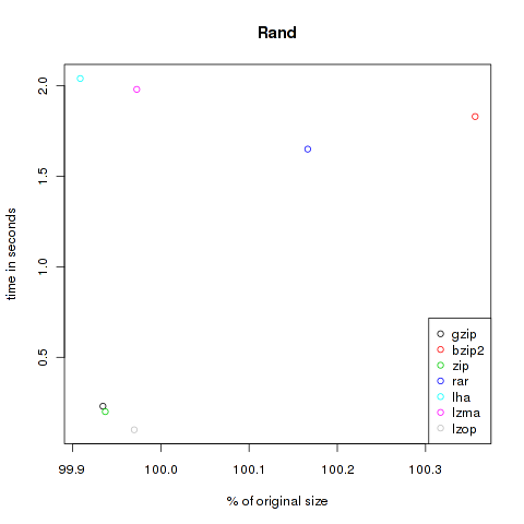
Rand
This category is just to test random generators. Compressing random content shouldn’t decrease the size of the files. Here I used two files from random.org and dumped some bytes from /dev/urandom. 4.198.400 Bytes.
| Method | Compressed Size | % of original | Time in s |
|---|---|---|---|
| gzip | 4.195.646 | 99.93 | 0.23 |
| bzip2 | 4.213.356 | 100.36 | 1.83 |
| zip | 4.195.758 | 99.94 | 0.2 |
| rar | 4.205.389 | 100.17 | 1.65 |
| lha | 4.194.566 | 99.91 | 2.04 |
| lzma | 4.197.256 | 99.97 | 1.98 |
| lzop | 4.197.134 | 99.97 | 0.1 |
Everything
All files of the previous catergories compressed together. Since the categories aren’t of same size it is of course not really fair. Nevertheless it might be interesting. All files together require 355.971.825 Bytes.
| Method | Compressed Size | % of original | Time in s |
|---|---|---|---|
| gzip | 294.793.255 | 82.81 | 20.43 |
| bzip2 | 290.093.007 | 81.49 | 141.89 |
| zip | 313.670.439 | 88.12 | 23.78 |
| rar | 305.083.648 | 85.70 | 246.63 |
| lha | 315.669.631 | 88.68 | 64.81 |
| lzma | 283.475.568 | 79.63 | 258.05 |
| lzop | 307.644.076 | 86.42 | 7.89 |

Conclusion
As you can see, the violet lzma-dot is always located at the left side, meaning very good compression. But unfortunately it’s also always at the top, so it’s very slow. But if you want to compress files to send it via mail you won’t bother about longer compression times, the file size might be the crucial factor. At the other hand black, green and grey (gzip, zip and lzop) are often found at the bottom of the plots, so they are faster but don’t decrease the size that effectively.
All in all you have to choose the method on your own. Also think about compatibility, not everybody is able to unpack lzma or lzop.. My upshot is to use lzma if I want to transfer data through networks and for attachments to advanced people, and to use gzip for everything else like backups of configs or mails to windows user.
A Synapt - or something like that...
March 28th, 2011As I mentioned, our university bought a Synapt G2 HDMS with an upstream 2D-UPLC. And what should I say, we are not amused.. But let’s start with the good things.
The innovative
As far as I know Waters is the first manufacturer who joined the IMS- and QTOF-technologies to combine all well known benefits from the QTOF instruments plus the advantages of separating ions by their shape and size. They developed a Triwave technology, consisting of a trap cell, the new IMS cell and a transfer cell. Trap and transfer cell are able to fragment the ions, so you can produce fragment ions before and/or after separation by ion mobility. Producing fragments is nothing new, most of the MS instruments out there are able to do so. The innovation is located at the IMS. In front of this cell you can find a Helium chamber, working as a gate. During an IMS cycle no further ions are able to pass this gate. The IMS cell itself is flooded with nitrogen. Ions that want to pass this cell interact with those nitrogen molecules, so they will slow down. The bigger the ionshape the higher the braking force of nitrogen.
The energy inside isn’t that high that ions decay to further fragments. The energy beam transporting the ions through the IMS cell can be understood as a wave. You can define the wave height and the velocity to effectively separate your present ions. Don’t ask me why the call it height and velocity, and not amplitude and frequency, but what ever ;-) Waters provides some videos to visualize this technology, and here you can find some smart pictures of the Triwave system in a Synapt.
If you now think about an 4m IMS cell take a look at figures 2 and 3, it’s a bit more than half of a keyboard length.
The other very cool thing is their UPLC. Never seen a two-dimensional LC! In one dimension you’ll find one C18 column to separate your complex sample. With this UPLC you can also trap species in columns with different pH values, so they are also separated by their different pH-column-interactions. This is really great if you want to analyze incredible complex samples.
Looking at these very cute technologies, what are we arguing about!?
The annoying
First of all, the sales process did not run as smoothly as one might expect and took a very long time. But since I wasn’t involved I can’t tell you anymore.
The first thing we recognized when the machine arrived was a 4kDa RF generator. But we ordered a 8kDa generator! How could this happen? Waters guarantees that each instrument will be tested before it leaves their plant.. The next thing followed immediately. All configurations of the EPC were lost.. While delivering! Seems that the postman is a pickpocket..
And, to carry it too far, within the first tests the IMS cell crashed unrecoverably, have a look at figures 2 and 3. So we had to wait for a new one from Manchester. To also name the positives, the shipment took less then one day.
Even if some innocent people think they can operate a MS (who told them!? hope they got paid), it took the technicians about six weeks to get the Synapt operating… Always arguing about nano-ESI… They had big problems to install the 2D-LC, the peaks still look freaky tailing… (I don’t want to run down the technicians, they were always very committed and tried to help us as far as possible!)
Ok, so far, all is not lost if we can operate now! But can we?
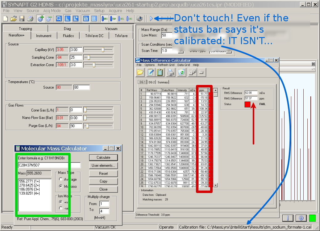
For calibration you need exact masses. Calculating masses of molecules isn’t a problem for waters, but adding a proton (H+) is! Instead of a proton they add a hydrogen (H+ + e-)!? Assume you want to calibrate with Leucine Enkephaline (Leu-Enk). Leu-Enk is a peptide whose sequence is Tyr-Gly-Gly-Phe-Leu (C28H37N5O7) with a mass of \(555.269297\text{u}\). Adding a proton results in a single charged ion with a mass of (Adam Ries told us!): \(555.269297\text{u} + 1.007276\text{u} = 556.276573\text{u}\) When they add a hydrogen their mass becomes: \(555.269297\text{u} + 1.007825\text{u} = 556.277122\text{u}\), that’s a diff of \(0.000549\text{u}\) (it’s the mass of an electron). Seems to be small, but think in ppm: \(\frac{0.000549\text{u} \cdot 10^6 }{555.269297\text{u}} \approx 0.9887\text{ppm}\). A systematic discrepancy of almost 1 ppm for an instrument specified for 1 ppm precision. Just because of a calculation error! And things become even worse at higher charge states, compare to the green part of figure 4. Do we (stupid scientists) really have to help them (MS specialists) summing up?
Playing a bit with the machine we figured out, that it is not constructed for static measurements. We had to be creative to get some backpreasure. You also have to unmount the whole static source block to load the needle with sample. Yes, they have these fluidics, but we have samples of few μl. Ok, prepared the system with some more handwork for static measurments, the results were disgusting. The acquired spectra had errors of more than 50 ppm (read box in figure 4)!? Calling Waters we found out that this is a known bug… Even if the acquisition-window leads to believe that the machine is calibrated and provides a button to start an acquisition, acquisitions have to be started from the MassLynx sample list. Not enough hands for face palms! It’s very complicated to create a sample for each static measurement, since you have to create a new method for each sample! Also the technicians weren’t able to tell us a lot about the working principle with IMS. But we, of course, want to try some things before running 9h experiments through LC just to see that the actual parameters for the IMS are crap…
Last but not least, they are not very cooperative when we call to tell them their faults…
If the policy of their company doesn’t change I don’t believe that we buy further instruments from Waters… Looking at the price for the machine I think buying some big cars to impress the girls would have been a much better investment ;-)
Very first time with a Synapt
February 26th, 2011Yesterday I had my first date with a SYNAPT™ from Waters. A workgroup from the biocentrum bought one, this week it was delivered.
So what’s a SYNAPT™? I would say it’s actually the cream of the crop of mass spectrometry platforms. It primarily differs from other platform in the feature of separation in terms of ion mobility.
Common platforms like QTof’s might distinguish between two peptides based on their mass, so they are separated in an Quadrupole, their mass over charge (m/z) is afterwards measured by their TOF. But there is a challenge with isobars. Since they have the same mass you’ll only get one peak for all of them. You are not able to differentiate between different elementary compositions with equal masses.
Waters now brings light to the dark. They developed a very new dimension of discovery. Their Triwave™ Technology allows you to dissolve different shapes of ions with equally mass. Actually I can’t tell you how it works, but take two sheets of paper, crush one of it and throw both out of your window. You see, there are some physics that let one of these papers reach the ground faster than the other one. With the SYNAPT™ you are able to distinguish between elements in your sample based on their shape.
With the upstream UPLC a species gives a peak in an spectrum, specified by retention time, m/z, shape and intensity. A new challenge to analyze and evaluate the resulting data.
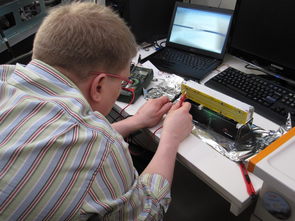
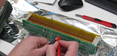
(Fortunately) there was a small problem with the machine, so I was able to take a look inside. It was amazing to see the guts of this big box, stuffed with filigree technique!!
I think I felt in love with this machine.. Bad news for my wife, but that’s life ;-)