binfalse

Stretching @YOKOFAKUN

June 14th, 2011

I’m following Pierre Lindenbaum both on twitter and on his blog. I love his projects, but I don’t like the layout of his blog, so I created a user-script to make the style more comfortable.

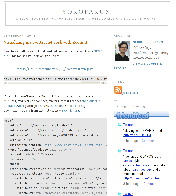
The problem is the width of his articles. The content is only about 400 pixel. Since Pierre often blogs about programming projects his articles are very code-heavy, but lines of code are usually very long and word-wrap isn’t appropriate in this case. So you have to scroll a lot to get the essential elements of his programs, see figure 1 as example from the article Visualizing my twitter network with Zoom.it.

The Firefox extension Greasemonkey comes to help. As you might know, with this extension you can easily apply additional JavaScript to some websites. So I created a so called user-script to stretch his blog. By default the main content is stretched by 200 pixel, so it’s about 1.5 times wider, see figure 2.

The code:

// ==UserScript==
// @name           YOKOFAKUN stretcher
// @namespace      binfalse.de
// @description    stretch the content on plindenbaum.blogspot.com
// @include        *plindenbaum.blogspot.com/*
// ==/UserScript==

var stretchPixels = 200;
var removeFriendFeed = false;
var toChange = new Array ("header-wrapper", "outer-wrapper", "main-wrapper");


// thats it, don't change anything below
// unless you know what you're doing!


function addCSS (css)
{
  var head = document.getElementsByTagName ('head') [0];
  if (!head)
    return;
  var add = document.createElement ('style');
  add.type = 'text/css';
  add.innerHTML = css;
  head.appendChild (add);
}

for (var i = 0; i < toChange.length; i++)
{
  var element = document.getElementById (toChange[i]);
  if (!element)
    continue;
  var org = parseInt (document.defaultView.getComputedStyle(element, null).getPropertyValue("width"));
  if (!org)
    continue;
  addCSS ('#' + toChange[i] + '{width: ' + (org + stretchPixels) + 'px}');
}

if (removeFriendFeed)
{
  var friendfeed = document.getElementById ('HTML3');
  if (friendfeed) friendfeed.parentNode.removeChild (friendfeed);
}

I also added a small feature to hide the friendfeed widget, I don’t like it ;-)

If you have installed Greasemonkey you just have to click the download-link below and Greasemonkey will ask if you want to install the script. To stretch the site by more/less pixel just change the content of the first variable to match your display preferences. If you set removeFriendFeed to true the friendfeed widget will disappear. So far, have fun with his articles!

Download: JavaScript: yokofakun_stretcher.user.js (Please take a look at the man-page. Browse bugs and feature requests.)

Apache: displaying instead of downloading

June 5th, 2011

When I found an interesting script and just want to see a small part of it I’m always arguing why I have to download the full Perl or Bash file to open it in an external program… And then I realized the configuration of my web servers is also stupid.

See for example my monitoring script to check the catalysts temperature. Till today you had to download it to see the content. To instead display the contents I had to tell the apache it is text. Here is how you can achieve the same.

First of all you need to have the mime module enabled. Run the following command as root:

a2enmod mime

You also need to have the permissions to define some more rules via htaccess . Make sure your Directory directive of the VirtualHost contains the following line:

AllowOverride All

Now you can give your web server a hint about some files. Create a file with the name .htaccess in the directory containing the scripts with the content:

<IfModule mod_mime.c>
 AddType text/plain .sh
 AddType text/plain .pl
 AddType text/plain .java
 AddType text/plain .cpp
 AddType text/plain .c
 AddType text/plain .h
 AddType text/plain .js
 AddType text/plain .rc
</IfModule>

So you defined scripts ending with .sh and .pl contain only plain text. Your firefox will display these files instead asking for a download location…

Btw. the .htaccess file is recursive, so all directories underneath are also affected and you might place the file in one of the parent directories of your scripts to change the behavior for all scripts at once. I installed it to my wordpress uploads folder.

Displaying compounds with WebGL

June 4th, 2011

After publishing my last article about OPSIN I was interested in using HTML5 techniques to display chemical compounds and found a nice library: ChemDoodle.

With ChemDoodle it’s very easy to display a molecule. Just download the libs and import them to your HTML code:

<script type="text/javascript" src="path/to/ChemDoodleWeb-libs.js"></script>
<script type="text/javascript" src="path/to/ChemDoodleWeb.js"></script>

To display a compound you need its representation as MOL file, include it in less than 10 lines:

<script type="text/javascript">
  var app = new ChemDoodle.TransformCanvas3D('transformBallAndStick', 500, 500);
  app.styles.set3DRepresentation('Stick');
  app.styles.backgroundColor = 'white';
  var molFile = '\n  Marvin  02080816422D          \n\n 14 15  0  0  0  0            999 V2000\n   -0.7145   -0.4125    0.0000 C   0  0  0  0  0  0  0  0  0  0  0  0\n   -0.7145    0.4125    0.0000 N   0  0  0  0  0  0  0  0  0  0  0  0\n    0.7145   -0.4125    0.0000 C   0  0  0  0  0  0  0  0  0  0  0  0\n    0.7145    0.4125    0.0000 C   0  0  0  0  0  0  0  0  0  0  0  0\n    0.0000   -0.8250    0.0000 N   0  0  0  0  0  0  0  0  0  0  0  0\n    0.0000    0.8250    0.0000 C   0  0  0  0  0  0  0  0  0  0  0  0\n    1.4992    0.6674    0.0000 N   0  0  0  0  0  0  0  0  0  0  0  0\n    1.4992   -0.6675    0.0000 N   0  0  0  0  0  0  0  0  0  0  0  0\n    1.9841    0.0000    0.0000 C   0  0  0  0  0  0  0  0  0  0  0  0\n   -1.4289   -0.8250    0.0000 O   0  0  0  0  0  0  0  0  0  0  0  0\n    0.0001    1.6500    0.0000 O   0  0  0  0  0  0  0  0  0  0  0  0\n    0.0001   -1.6500    0.0000 C   0  0  0  0  0  0  0  0  0  0  0  0\n    1.7541    1.4520    0.0000 C   0  0  0  0  0  0  0  0  0  0  0  0\n   -1.4289    0.8250    0.0000 C   0  0  0  0  0  0  0  0  0  0  0  0\n 10  1  2  0  0  0  0\n  1  2  1  0  0  0  0\n 14  2  1  0  0  0  0\n  8  3  1  0  0  0  0\n  4  3  2  0  0  0  0\n  7  4  1  0  0  0  0\n  1  5  1  0  0  0  0\n  5  3  1  0  0  0  0\n 12  5  1  0  0  0  0\n  6  2  1  0  0  0  0\n  6  4  1  0  0  0  0\n 11  6  2  0  0  0  0\n  9  7  1  0  0  0  0\n 13  7  1  0  0  0  0\n  9  8  2  0  0  0  0\nM  END\n';
  var molecule = ChemDoodle.readMOL(molFile, 1);
  app.loadMolecule(molecule);
</script>

Here is a sample with caffeine:

If your browser is able to display WebGL you should see a stick-model. Use your mouse to interact. Very easy to use! Of course you can load the MOL data from a file, but that is beyond the scope of this article.

Benefit of standardization: OPSIN

June 3rd, 2011

Just read about a new tool to parse chemical names from systematic IUPAC nomenclature.

OPSIN (Open Parser for Systematic IUPAC nomenclature) is an open source IUPAC nomenclature parser. The IUPAC provides some rules to name chemical compounds, you may have learned some of them in your first course of organic chemistry.

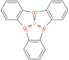
The web interface also comes with an API to generate a 2D picture of the parsed compound. You can speak to the API by calling the image via http://opsin.ch.cam.ac.uk/opsin/IUPAC-NAME.png . For example to get an image for 2λ6,2’,2’‘-spiroter[[1,3,2]benzodioxathiole] just follow these instructions and you’ll get an image like this:

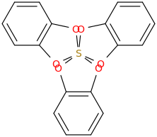
Very smart, isn’t it? Using the web interface they also provide InChI and SMILES strings and a CML definition.

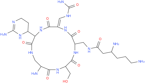
It’s not limited to simple molecules, I’ve tried some more complex names, for example 3,6-diamino-N-[[15-amino-11-(2-amino-3,4,5,6-tetrahydropyrimidin-4-yl)-8- [(carbamoylamino)methylidene]-2-(hydroxymethyl)-3,6,9,12,16-pentaoxo- 1,4,7,10,13-pentazacyclohexadec-5-yl]methyl]hexanamide:

What should I say, I’m impressed! You can download the tool at bitbucket or use the web interface.

R for the web

May 28th, 2011

There is a nice R module for apache: rApache. So you can easily publish statistics.

To install rApache first install the following packages from the Debian/Ubuntu repository:

aptitude install apache2 apache2-mpm-prefork apache2-prefork-dev r-base-dev

So the basics are done. Lets install rApache. Grab the latest version:

wget http://biostat.mc.vanderbilt.edu/rapache/files/rapache-latest.tar.gz

extract the contents and cd into it. The installation process should be clear, I had to give a hint for the apxs2 location:

./configure --with-apxs=/usr/bin/apxs2
make
make install

To notify apache about the new module you need to create two more files. First one is /etc/apache2/mods-available/r.conf :

<Location /R>
ROutputErrors
SetHandler r-script
RHandler sys.source
</Location>

<Location /RApacheInfo>
SetHandler r-info
</Location>

Now all files in /R are assumed to be R-scripts, in /RApacheInfo you’ll find some information about your installation. The second file is /etc/apache2/mods-available/r.load :

LoadModule R_module /usr/lib/apache2/modules/mod_R.so

This file just defines which lib to load. To finish the installation you need to load the rApache module and restart the webserver via:

a2enmod r
/etc/init.d/apache2 restart

That’s it. You can test whether all was successful by browsing to localhost/RApacheInfo, hopefully you’ll see some config stuff. To prepare some own tests create a directory /var/www/R (assuming your document-root is /var/www ) and paste something like this in a file called test :

y = rnorm(100)
print(y)

Browsing to localhost/R/test you should see something like this:

[1] -0.4969626136 -0.0004799614  1.3858672447 -0.1888848545  0.5577465024
  [6] -0.6463581808  1.3594363388  1.8160182284 -1.8602721944  0.3249432873
 [11]  1.0861606647 -0.5075055497 -0.5152062853  0.4851131375  0.2924883195
 [16] -0.5542238124  1.2741001461  0.2627202474 -0.8986869795 -0.8628182849
 [21] -0.0788598913  0.4843055866 -0.2747585510 -1.1928500793  1.6193763442
 [26]  0.3452218627  0.9518228897 -0.5858433386  1.9585346877 -0.2582043114
 [31] -1.7989436202  1.2713761553  0.9045031014 -0.3456065867  0.3739555330
 [36]  0.7512315203 -0.5289340037 -0.7700091217 -1.5103278314 -1.5195628428
 [41] -0.8100795062  1.1027597227  0.0194147933  0.7819879165 -0.3914496199
 [46] -0.4650911293  0.5889685176 -0.9659270213  1.0570030616 -0.0657166412
 [51] -0.2077095857  0.6421821337 -0.1911934111 -3.1567052058  0.2704713187
 [56] -0.5154689593  0.0923834868 -1.2100314635  0.6693369266 -1.2093881229
 [61]  1.6755264101  1.2151146432  0.6683583636 -0.2982231602  1.4830922366
 [66]  1.6505026636 -0.1769048244  0.3516470621 -0.0053594481 -0.3776870673
 [71] -0.4797554602  1.2207702646  1.2762816419 -2.6137169267 -1.4423704831
 [76] -0.4251822440  0.8007722424 -0.4985947758 -2.0685396392 -1.6844317212
 [81] -0.2509955532  0.7906569225 -0.1259848747 -0.1352738978 -1.4943405839
 [86] -2.4272199144 -0.5778250558  1.2579971393 -1.0476874144  0.2305160769
 [91] -0.2920446292  0.1823053837  1.8858770756  1.4158084170 -1.2539321864
 [96]  1.2667650232  0.1272379338  1.2726069769  0.8745111042  0.3848103655

To create a graphic you need to change the content type to an image type. A small example might give you an idea:

setContentType ("image/png")
temp <- tempfile ()
y = rnorm (100)
png (temp, type="cairo")
plot (1:100, y, t='l')
dev.off ()
sendBin (readBin (temp, 'raw', n=file.info(temp)$size))
unlink (temp)

Reload the page and you’ll see a more or less nice plot :-P That’s it for the moment, for a more interactive interface take a look at the ggplot2 mod.

Download: R: web-image.R (Please take a look at the man-page. Browse bugs and feature requests.)

Martin Scharm

stuff. just for the records.

Do you like this page?
You can actively support me!